Instrument driver

Once srsinst.rga is installed to your computer, you can use it to control and acquire data from SRS RGAs in various Python environments, such as Python interpreter console, Jupyter notebook, context-sensitive editors, or just to write Python scripts.

Here we use the Python interpreter in interactive mode to show how to use RGA100 class to communicate with an RGA.

When you start Python from the command line, the ‘>>>’ prompt is waiting for your input.

C:\rga>python
C:\PyPI\rga>C:\Users\ckim\AppData\Local\Programs\Python\Python38\python.exe
Python 3.8.3 (tags/v3.8.3:6f8c832, May 13 2020, 22:37:02) [MSC v.1924 64 bit (AMD64)] on win32
Type "help", "copyright", "credits" or "license" for more information.
>>>

Connecting to an RGA

From the prompt, import RGA100 class and connect to an RGA.

>>> from srsinst.rga import RGA100
>>> rga1 = RGA100('serial', 'COM3', 28800)  # This is for a Windows computer
>>> rga1.check_id()
('SRSRGA200', '19161', '0.24')

In the case shown above, the RGA is connected to the serial port, COM3 on a Windows computer. Note that RGA 100 series only connects with the baud rate of 28800.

The check_id() method reads the identification string from the RGA and adjust the Scans component depending on the highest mass.

Note that the serial port notation with a Linux computer is different from that of a Windows computer.

>>> rga2 = RGA100('serial', /dev/ttyUSB0', 28800)  # for Linux serial communication
>>>

If your RGA is equipped with the RGA ethernet adapter (REA), it can be connected over Ethernet.

>>> rga3 = RGA100('tcpip', '192.168.1.100', 'admin',' admin')
>>>

You have to know the IP address, the user name and the password of the REA, to connect to an REA equipped RGA.

A general usage of RGA100 class can be simplified as:

Create an instance of RGA100 class

Connect to an RGA

Use it

Disconnect from it

>>>
>>> rga3 = RGA100()
>>> rga3.connect('tcpip','192.168.1.100','admin','admin')
>>> rga3.check_id()
('SRSRGA200', '19161', '0.24')
>>> rga3.disconnect()
>>>

Navigating through `RGA100` class

RGA100 class contains many attributes and methods to interact with an RGA. RGA100 is the root component that contains many subcomponents. Each component has its subcomponents, commands and class methods. Components can be compared as directories in the computer file structure, and commands and methods as files.

The dir attribute of a component shows what it holds in the dictionary format.

Here is the output of the dir attribute of the RGA100 instance.

>>> rga1.dir
{'components': {'ionizer': 'instance of Ionizer', 'filament': 'instance of Filament', 'cem': 'instance of CEM', 'scan': 'instance of Scans200', 'qmf': 'instance of QMF', 'pressure': 'instance of Pressure', 'status': 'instance of Status'}, 'commands': {}, 'methods': ['connect', 'check_id', 'get_status', 'handle_command', 'reset', 'check_head_online', 'get_max_mass', 'calibrate_all', 'calibrate_electrometer', 'disconnect', 'is_connected', 'set_term_char', 'get_term_char', 'send', 'query_text', 'query_int', 'query_float', 'get_available_interfaces', 'get_info', 'connect_with_parameter_string']}
>>>

Well, the output of a dictionary in one line is not the best way to look into it. Let’s use the pretty printer.

>>> import pprint  # Use Data Pretty Printer
>>> pp = pprint.PrettyPrinter(indent=4, sort_dicts=False)
>>> pp.pprint( rga1.dir )
{   'components': {   'ionizer': 'instance of Ionizer',
                      'filament': 'instance of Filament',
                      'cem': 'instance of CEM',
                      'scan': 'instance of Scans200',
                      'qmf': 'instance of QMF',
                      'pressure': 'instance of Pressure',
                      'status': 'instance of Status'},
    'commands': {},
    'methods': [   'connect',
                   'check_id',
                   'get_status',
                   'handle_command',
                   'reset',
                   'check_head_online',
                   'get_max_mass',
                   'calibrate_all',
                   'calibrate_electrometer',
                   'disconnect',
                   'is_connected',
                   'set_term_char',
                   'get_term_char',
                   'send',
                   'query_text',
                   'query_int',
                   'query_float',
                   'get_available_interfaces',
                   'get_info',
                   'connect_with_parameter_string']}
>>>

It looks still overwhelming, because it has so many items: 7 subcomponents (ionizer, filament, cem, qmf, pressure, status) and 20 methods.

As long as you can find what you want to use, it helps you to spot it and get the correct name.

Setting up `ionizer`

Let’s take a look into the ionizer component.

>>> pp.pprint( rga1.ionizer.dir )
{   'components': {},
    'commands': {   'electron_energy': ('RgaIntCommand', 'EE'),
                    'ion_energy': ('RgaIonEnergyCommand', 'IE'),
                    'focus_voltage': ('RgaIntCommand', 'VF'),
                    'emission_current': ('RgaFloatCommand', 'FL')},
    'methods': ['get_parameters', 'set_parameters']}
>>>

It contains commands and methods to configure the ionizer of the RGA. Commands are defined using the Python descriptor to encapsulate raw RGA remote commands.

Each command item is defined as:

‘command name’: (‘Command class name’, the raw ‘RGA remote command’ that can be found in the RGA manual).

For example, the command electron_energy is defined using RgaIntCommand and it encapsulate the RGA remote command ‘EE’.

You can configure the ionizer parameters in various ways.

>>> rga1.ionizer.get_parameters()
(70, 12, 90)     # tuple of (electron energy, ion energy, focus voltage)
>>> rga1.ionizer.electron_energy
70
>>> rga1.ionizer.electron_energy = 69
>>> rga1.ionizer.electron_energy
69
>>> rga1.ionizer.ion_energy
12
>>> rga1.ionizer.ion_energy = 8
>>> rga1.ionizer.ion_energy
8
>>> rga1.ionizer.focus_voltage
90
>>> rga1.ionizer.focus_voltage = 89
>>> rga1.ionizer.focus_voltage
89
>>> rga1.ionizer.get_parameters()
(69, 8, 89)
>>> rga1.ionizer.set_parameters()  # set to default
0
>>> rga1.ionizer.get_parameters()
(70, 12, 90)
>>>

By defining a command as Python descriptor, it can be used as an attribute instead of using raw communication functions in RGA100 class with RGA raw commands.

>>> rga1.query_int('EE?')  # equivalent to 'rga1.ionizer.electron_energy'
70
>>> rga1.query_int('EE69') # equivalent to 'rga1.ionizer.electron_energy = 69'
1
>>> rga1.query_int('EE?')
69
>>>

Turning `filament` on/off

You can turn the filament on or off, by adjusting the emission current in the ionizer component.

>>> rga1.ionizer.emission_current
0.3852
>>> rga1.ionizer.emission_current = 1.0
>>> rga1.ionizer.emission_current
1.0065

There is also the dedicated filament component.

>>> pp.pprint( rga1.filament.dir )
{   'components': {},
    'commands': {},
    'methods': ['turn_on', 'turn_off', 'start_degas']}
>>>
>>> print( rga1.filament.turn_on.__doc__ )

        Turn on filament to the target emission current

        Parameters
        -----------
            target_emission_current : int, optional
                Default is 1.0 mA

        Returns
        --------
            error_status : int
                Error status byte

>>>
>>> rga1.ionizer.emission_current
0.0
>>> rga1.filament.turn_on()
0
>>> rga1.ionizer.emission_current
1.0076
>>> rga1.filament.turn_off()
0
>>>

Setting up detector

You can select the Faraday cup detector by setting CEM voltage to 0, and select Channel electron multiplier (CEM) detector and CEM voltage to a positive value.

>>> pp.pprint( rga1.cem.dir )
{   'components': {},
    'commands': {   'voltage': ('RgaIntCommand', 'HV'),
                    'stored_voltage': ('FloatNSCommand', 'MV'),
                    'stored_gain': ('RgaStoredCEMGainCommand', 'MG')},
    'methods': ['turn_on', 'turn_off']}
>>> print( rga1.cem.turn_on.__doc__ )

        Set CEM HV to the stored CEM voltage

>>> rga1.cem.stored_voltage
1043.0
>>> rga1.cem.voltage
0
>>> rga1.cem.turn_on()
>>> rga1.cem.voltage
1035
>>> rga1.cem.voltage = 0
>>> rga1.cem.voltage
0

Setting up a scan

Getting mass spectra is the core task of an RGA. All the functionality of acquiring mass spectra resides in Scans class.

Let’s take a look what are available with the instance of Scans class with the dir attribute.

>>> pp.pprint( rga1.scan.dir )
{   'components': {},
    'commands': {   'initial_mass': ('IntNSCommand', 'MI'),
                    'final_mass': ('IntNSCommand', 'MF'),
                    'speed': ('IntNSCommand', 'NF'),
                    'resolution': ('IntNSCommand', 'SA'),
                    'total_points_analog': ('IntGetCommand', 'AP'),
                    'total_points_histogram': ('IntGetCommand', 'HP')},
    'methods': [   'set_callbacks',
                   'set_data_callback_period',
                   'get_data_callback_period',
                   'get_max_mass',
                   'get_parameters',
                   'set_parameters',
                   'read_long',
                   'get_mass_axis',
                   'get_analog_scan',
                   'get_histogram_scan',
                   'get_multiple_mass_scan',
                   'get_single_mass_scan',
                   'set_mass_lock',
                   'get_partial_pressure_corrected_spectrum',
                   'get_peak_from_analog_scan']}
>>>

To set up a scan, we have to specify the initial mass, final mass, scan speed, and resolution (steps per AMU).

>>> rga1.scan.get_parameters()
(2, 50, 3, 20)
>>> rga1.scan.initial_mass = 1
>>> rga1.scan.final_mass = 65
>>> rga1.scan.speed = 4
>>> rga1.scan.resolution = 10
>>> rga1.scan.get_parameters()
(1, 65, 4, 10)
>>> rga1.scan.set_parameters(10, 50, 3, 20)
>>> rga1.scan.get_parameters()
(2, 50, 3, 20)
>>>

Acquiring a histogram scan

>>> rga1.scan.set_parameters(10, 50, 3, 20)
>>> histogram_mass_axis = rga1.scan.get_mass_axis(for_analog_scan=False)
>>> histogram_mass_axis
array([10., 11., 12., 13., 14., 15., 16., 17., 18., 19., 20., 21., 22.,
       23., 24., 25., 26., 27., 28., 29., 30., 31., 32., 33., 34., 35.,
       36., 37., 38., 39., 40., 41., 42., 43., 44., 45., 46., 47., 48.,
       49., 50.])
>>>
>>> histogram_spectrum = rga1.scan.get_histogram_scan()
>>> histogram_spectrum
array([ 211.,  175.,   56.,   24.,  249.,  129.,  213.,  303.,  639.,
        533.,  217.,  191.,  206.,  179.,  256.,  116., -116.,  222.,
        343.,  240.,  206.,  249.,  347.,  483.,   20.,  -65.,  104.,
        249.,  179.,  307.,  239.,  245.,  347.,  262.,  312.,  226.,
        307.,  271.,  468.,  226.,  201.])

Acquiring a analog scan

>>> rga1.scan.set_parameters(1, 50, 3, 20)
>>> mass_axis = rga1.scan.get_mass_axis(for_analog_scan=True)
>>>
>>> spectrum = rga1.scan.get_analog_scan()
>>> spectrum_in_torr = rga1.scan.get_partial_pressure_corrected_spectrum(spectrum)

Saving a spectrum to a file

>>> with open('spectrum.dat', 'w') as f:
...    for x, y in zip(mass_axis, spectrum_in_torr):
...        f.write('{:.2f} {:.4e}\n'.format(x, y))

Plot a spectrum with matplotlib 

>>> import matplotlib.pyplot as plt
>>> plt.plot(mass_axis, spectrum_in_torr)
>>> plt.show()

It will bring up a plot showing an analog scan spectrum.

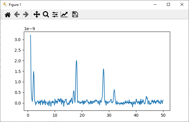
As a summary, the following script is put together to get an analog scan plot from the beginning.

import matplotlib.pyplot as plt
from srsinst.rga import RGA100

rga1 = RGA100('serial','COM3', 28800)

rga1.filament.turn_on()
rga1.cem.turn_off()
rga1.scan.set_parameters(1, 50, 3, 20)  # (initial mass, final mass, scan speed, resolution)
mass_axis = rga1.scan.get_mass_axis(True)  # True for analog scan, False for histogram scan
spectrum = rga1.scan.get_analog_scan()
spectrum_in_torr = rga1.scan.get_partial_pressure_corrected_spectrum(spectrum)
rga1.disconnect())

plt.plot(mass_axis, spectrum_in_torr)
plt.show()