Example project
When you run the srsgui application, the console window shows
where Python is running from, and where srsgui is located.
If you go into the directory where srsgui resides, you can find
the ‘examples’ directory. When you find a .taskconfig file in “oscilloscope example”
directory, Open the file from the File/Open Config menu of srsgui application.
If you plan to modify files in the project, you should copy the whole examples directory
to a separate location (outside of the virtual environment or Python directory;
e.g. where you usually keep your documents for programing).
Then you can open and modify the .taskconfig file in the copied directory
without any worry of corrupting or losing the original files.
As an example project for srsgui, I wanted to use ubiquitous measurement
instruments with remote communication available. I happened to have an
oscilloscope and a function generator (more specifically, a clock generator)
on my desk:
I built a project that controls both instruments and
captures output waveform from the clock generator with the oscilloscope,
calculates an FFT, and displays the waveforms in the srsgui application.
Any oscilloscope and function generator will work for this example.
If you are interested in srsgui, chances are you can find an oscilloscope
and a function generator somewhere in your building.
If you could not, don’t worry. Even without an any instruments, we can generate a
simulated waveform to demonstrate the usability of srsgui as an organizer for
Python scripts and GUI environment for convenient data acquisition and data visualization.
Directory structure
Let’s look at the directory structure of the project.
/Oscilloscope example project directory
    /instruments
        cg635.py
        sds1202.py
    /tasks
        identify.py
        plot_example.py
        ...

    oscilloscope example project.taskconfig
This file structure follows the guideline described in Creating file structure for a project. We have two instrument driver scripts for SDS1202XE and CG635 in the subdirectory called instruments, five task scripts in the subdirectory called tasks, plus a configuration file in the project root directory.
Project configuration file
The structure of a .taskconfig file is simple and explained in Populating the .taskconfig file
1name: Srsgui Example - Oscilloscope and Clock Generator
2
3inst: cg,  instruments.cg635,   CG635
4inst: osc, instruments.sds1202, SDS1202
5
6task: *IDN test,                 tasks.idenfify,  Identify
7task: Plot example,              tasks.plot_example, PlotExample
8...
Instrument drivers
CG635
Let’s take a look into the instruments/cg635.py module. Even though it seems long, it has only 5 lines of non-comment code. If you have a CG635, congratulations! You can use the file as is. If you have any function generator that can change the output frequency, you can use it instead of the CG635 in the example. You change the class name and _IdString to match the instrument name, along with _term_char. Look up the command to change frequency, referring to the manual. Save the .py file with a (different) appropriate filename. Change the inst: line for cg in the .taskconfig file to match the module path and the class name that you created.
1from srsgui import Instrument
2from srsgui.inst import FloatCommand
3
4class CG635(Instrument):
5    _IdString = 'CG635'
6    frequency = FloatCommand('FREQ')
Without redefining available_interfaces class attribute, you can use serial communication only. If you want to use GPIB communication, you have to un-comment the available_interfaces in CG635 class.
from srsgui import SerialInterface, FindListInput
from srsinst.sr860 import VisaInterface

available_interfaces = [
    [   SerialInterface,
        {
            'COM port': FindListInput(),
            'baud rate': 9600
        }
    ],
    [   VisaInterface,
        {
            'resource': FindListInput(),
        }
    ],
]
You must install srsinst.sr860 for VisaInterface class, and PyVISA and its backend library, following PyVisa installation instruction.
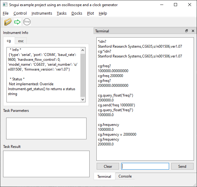
Once the CG635 (or your function generator) is connected, you will see the connection information in the instrument info panel, and you can use it in the terminal, as shown below.
To fix the ‘Not implemented’ warning,
Instrument.get_status()
needs to be redefined.
For example, we can override it as following:
def get_status(self):
    return 'Status: OK'
(If you are familiar with status bytes, you can override the get_status method to query the status byte(s) and return the relevant status information as you desire.)
We will use only one command .frequency, or its raw remote command, ‘freq’ in this example. Because ‘cg’ is the default instrument (the first instrument mentioned in the .taskconfig file), any raw remote command without the ‘cg:’ prefix will be sent to it. Both ‘*idn?’ and ‘cg:*idn?’ will return the same reply.
We use the prefix ‘cg:’ for raw remote command and the prefix ‘cg.’ for Python commands. In the terminal all attributes and methods of CG835 class can be used with prefix ‘cg.’. Because we defined frequency as a FloatCommand, we can also use the ‘cg.frequency’ property in the terminal. This means that the following are equivalent: - cg:freq 100.0 - cg.frequency 100
Furthermore, from a Python script, once get_instrument(‘cg’) has been called in a task class, you can use cg.frequency = 100 in the Python task code (or cg.frequency as the query form).
Actually you can use all the attributes and methods defined in the CG635 class and its super classes.
The cg.dir() method (where dir() is defined in Component class)
shows all the available components, commands, and methods available to an instance of the CG635 class.
This helps us to navigate through resources available with the class.
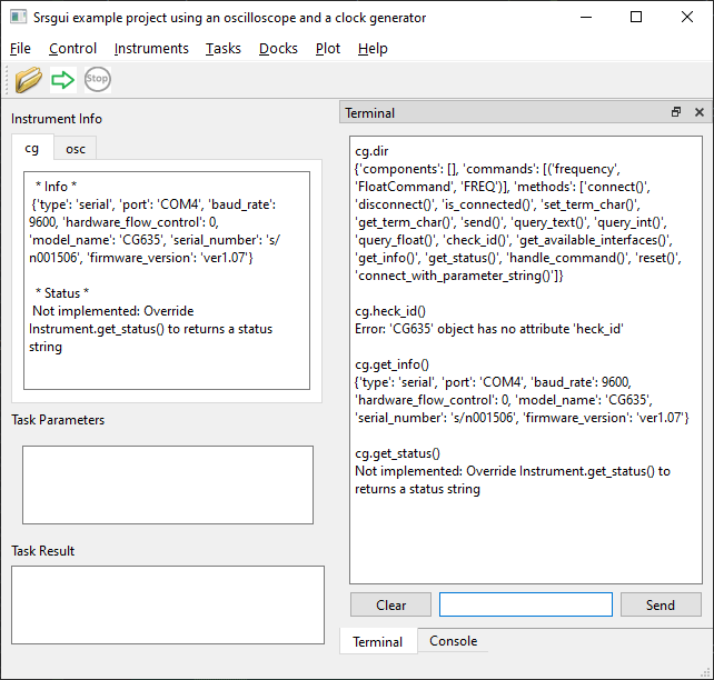
Cracking open the instrument manual and defining useful methods in an instrument class provides ease of instrument control from either the Terminal or from your task code, without having to remember the remote command mnemonics themselves.
SDS1202
Even though you may not have an SDS1202 oscilloscope that I happened to use for this example, I bet you can find an oscilloscope somewhere in your building. When you get a hold of one, it may have a USB connector only, like a lot of base model oscilloscopes do. This means you may have to use USB-TMC interface. In order to do that, you need to install PyVISA. You need to uncomment the available_interfaces of SDS1202 class, modify it to fit the specification of your oscilloscope, along with changing to the correct _IdString. Then you have to get waveform download working, which often involves recieving and properly parsing binary data (binary data is used to minimize the number of characters sent over the remote communication interface, thereby making data transfers of perhaps very lengthy waveforms relatively fast). If you are lucky, you can find a working Python snippet from judicious web search. If not, you have to decipher the programming manual of the oscilloscope. It may take time, but it will be very rewarding for your data acquisition skill-set improvement.
Other than the binary waveform download, most other commands for interacting with the oscilloscope will be standard ASCII-based text commands.
Note
With default available_interfaces of Instrument class, TcpipInterface should be used with port 5025.
The instrument driver for SDS1202 will work with 4 lines of code, just like the CG635, before adding the method to download waveforms from the oscilloscope. Add attributes and methods incrementally as you need to use more functions of the instrument.
 1import numpy as np
 2from srsgui import Instrument
 3
 4class SDS1202(Instrument):
 5    _IdString = 'SDS1202'
 6
 7    def get_waveform(self, channel):
 8        ...
 9
10    def get_sampling_rate(self):
11        ...
Once the oscilloscope is connected to the application, you can use the terminal to explore the oscilloscope.
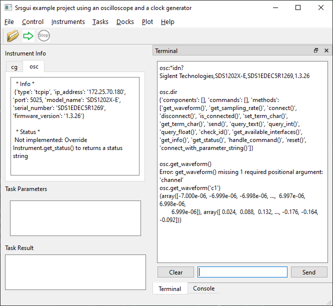
Because ‘osc’ is not the default instrument, you have to use the prefix ‘osc:’ with all the raw remote commands you send to the instrument. As shown with ‘osc.dir’, there are many methods available with ‘osc.’ Even osc.get_waveform() is available from the terminal. When you use a method incorrectly, the terminal kindly tells me that there is a missing argument in a function call. You can see osc.get_waveform(channel) returns two numpy arrays. What if you want to plot the data? As the methods you implement for interacting with your instruments and data grow in complexity, you may need to graduate from terminal-based interaction to task-based interaction. Read on.
Tasks
How to run a task
Start the srsgui application. You can see where the .taskconfig file is opened
from the console window (here).
If you made a copy of the original example from the srsgui
package directory, open it again from the correct directory.
If there are no error messages in the Console window, connect the function generator and the oscilloscope from the Instruments menu.
The overall structure of a task is described in Writing a task script section. There are 5 tasks are included in the example project. They gradually add more features on the top of the previous tasks. They are designed to showcase how to use the Task class.
Select the first task (*IDN test) from the Tasks menu and click the green arrow in the tool bar to run the task.
Identify task
The Identify task shows:
How to use module-level logger for Python logging in a task
How to use instruments defined in the configuration file
How to use text output to the console window
It is not much different from the bare bone structure shown in the Writing a task script section.
 1##!
 2##! Copyright(c) 2022, 2023 Stanford Research Systems, All rights reserved
 3##! Subject to the MIT License
 4##!
 5
 6from srsgui import Task
 7
 8
 9class Identify(Task):
10    """
11Query *IDN? to instruments, 'cg' and 'osc' \
12defined in the configuration file.
13    """
14
15    # No interactive input parameters to set before running
16    input_parameters = {}
17
18    def setup(self):
19        # To use Python logging
20        self.logger = self.get_logger(__file__)
21
22        # To use the instrument defined in .taskconfig file
23        self.cg = self.get_instrument('cg')
24        self.osc = self.get_instrument('osc')
25
26        # Set clock frequency tp 10 MHz
27
28        # frequency is define as FloatCommand in CG635 class
29        self.cg.frequency = 10000000
30        self.logger.info(f'Current frequency: {self.cg.frequency}')
31
32        # You can do the same thing with FloatCommand defined.
33        # You can use send() and query_float() with raw remote command
34        # self.cg.send('FREQ 10000000')
35        # self.current_frequency = self.cg.query_float('FREQ?')
36        # self.logger.info(self.current_frequency)
37
38    def test(self):
39        # You can use print() only with one argument.
40        print("\n\nLet's query IDs of instruments!!\n\n")
41
42        # Use query_text for raw remote command query returning string
43        cg_id_string = self.cg.query_text('*idn?')
44        osc_id_string = self.osc.query_text('*idn?')
45
46        self.logger.info(f"CG *IDN : {cg_id_string}")
47        self.logger.info(f"OSC *IDN : {osc_id_string}")
48
49    def cleanup(self):
50        # We have nothing to clean up
51        pass
Using self.logger sends the logging output to the console window, the master logging file in ~/task-results directory/mainlog-xx.txt.x, and to the task result data file located in ~/task-results/project-name-in-config-file/RNxxx directory.
With get_instrument you can get the instrument
defined in the configuration file in a task. Do not disconnect the instrument in the task!
Instrument Connectivity is managed at the srsgui application level.
This task highlights how remote command set and query transactions are simplified by defining
an attribute using srsgui.inst.commands module,
which is utilized in the CG635 class definition via the following line:
frequency = FloatCommand('FREQ')
This simple line makes it possible to set and query the cg.frequency without having to directly manipulate command or response strings.
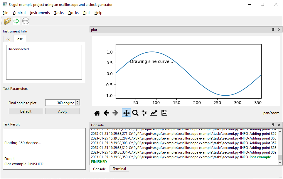
PlotExample task
The PlotExample task requires no instrument connections, and shows:
How to define
input_parametersfor interactive user input from the application input panelHow to use matplotlib figures for plotting data
How to send text output to the result window using
display_result()How to stop the task by checking
is_running().
 1##!
 2##! Copyright(c) 2022, 2023 Stanford Research Systems, All rights reserved
 3##! Subject to the MIT License
 4##!
 5
 6import time
 7import math
 8
 9from srsgui import Task
10from srsgui import IntegerInput
11
12
13class PlotExample(Task):
14    """
15Example to demonstrate the use of matplotlib plot in a task.
16No hardware connection is required.
17Generates a plot of y = sin(x) vs. x, \
18for x in the range [initial angle, final angle].
19    """
20
21    # Interactive input parameters to set before running
22    theta_init = 'initial angle'
23    theta_final = 'final angle'
24    input_parameters = {
25        theta_init: IntegerInput(0,' deg'),
26        theta_final: IntegerInput(360,' deg')
27    }
28    """
29    Use input_parameters to get parameters used in the task
30    """
31
32    def setup(self):
33
34        # Get a value from input_parameters
35        self.theta_i = self.get_input_parameter(self.theta_init)
36        self.theta_f = self.get_input_parameter(self.theta_final)
37
38        # Get the Python logging handler
39        self.logger = self.get_logger(__file__)
40
41        # Get the default Matplotlib figure
42        self.figure = self.get_figure()
43
44        # Once you get the figure, the followings are typical Matplotlib things to plot.
45        self.ax = self.figure.add_subplot(111)
46        self.ax.set_xlim(self.theta_i, self.theta_f)
47        self.ax.set_ylim(-1.1, 1.1)
48        x_txt = self.theta_i + 0.25*(self.theta_f - self.theta_i)
49        y_txt = 0.5
50        self.ax.text(x_txt, y_txt, 'Drawing sine curve...')
51        self.line, = self.ax.plot([0], [0])
52
53    def test(self):
54        print("\n\nLet's plot!\n\n")
55
56        x = []
57        y = []
58        rad = 180 / math.pi
59
60
61        for i in range(self.theta_i, self.theta_f+1, 1):
62            if not self.is_running():  # if the stop button is pressed, stop the task
63                break
64
65            self.logger.info(f'Adding point {i}')
66
67            # Display in the result panel
68            self.display_result(f'\n\nPlotting {i} degree...\n\n', clear=True)
69
70            # Add data to the Matplotlib line and update the plot
71            x.append(i)
72            y.append(math.sin(i / rad))
73            self.line.set_data(x, y)
74
75            # Figure update should be done in the main thread, not locally.
76            self.request_figure_update(self.figure)
77
78            # Delay a bit as if a sine function computation takes time.
79            time.sleep(0.01)
80
81    def cleanup(self):
82        self.display_result('Done!')
Using matplotlib with srsgui is straightforward if you are already familiar with its usage.
(Refer to matplotlib documentation).
- The important differences when using matplotlib in
srsguiare: You have to get the figure using get_figure(), rather than creating one on your own.
Plots are created during setup(), because it is a slow process. During test(), you simply update data using set_data() or similar methods for data update.
You must use request_figure_update() to redraw the plot, after set_data(). The event loop handler in the main application will update the plot at its earliest convenience.
ScopeCapture task
The ScopeCapture task uses the oscilloscope only. It gets the requested number of captures from user input, then repeats oscilloscope waveform capture and updates the waveform plot. It stops once the desired number of captures have been obtained, or when the Stop button is pressed. Waveforms are captured with 700000 points about every 0.2 seconds over TCP/IP communication.
 1##!
 2##! Copyright(c) 2022, 2023 Stanford Research Systems, All rights reserved
 3##! Subject to the MIT License
 4##!
 5
 6import time
 7from srsgui import Task
 8from srsgui import IntegerInput
 9
10
11class ScopeCapture(Task):
12    """
13It captures waveforms from an oscilloscope, \
14and plot the waveforms real time.
15    """
16
17    # Use input_parameters to set parameters before running
18    Count = 'number of captures'
19    input_parameters = {
20        Count: IntegerInput(100)
21    }
22
23    def setup(self):
24        self.repeat_count = self.get_input_parameter(self.Count)
25        self.logger = self.get_logger(__file__)
26
27        self.osc = self.get_instrument('osc') # use the inst name in taskconfig file
28
29        # Get the Matplotlib figure to plot in
30        self.figure = self.get_figure()
31
32        # Once you get the figure, the following are about Matplotlib things to plot
33        self.ax = self.figure.add_subplot(111)
34        self.ax.set_xlim(-1e-5, 1e-5)
35        self.ax.set_ylim(-1.5, 1.5)
36        self.ax.set_title('Scope waveform Capture')
37        self.x_data = [0]
38        self.y_data = [0]
39        self.line, = self.ax.plot(self.x_data,self.y_data)
40
41    def test(self):
42        prev_time = time.time()
43        for i in range(self.repeat_count):
44            if not self.is_running(): # if the Stop button is pressed
45                break
46
47            # Add data to the Matplotlib line and update the figure
48            t, v = self.osc.get_waveform('C1')  # Get a waveform of the Channel 1 from the oscilloscope
49            self.line.set_data(t, v)
50            self.request_figure_update()
51
52            # Calculate the time for each capture
53            current_time = time.time()
54            diff = current_time - prev_time
55            self.logger.info(f'Capture time for {len(v)} points of waveform {i}: {diff:.3f} s')
56            prev_time = current_time
57
58    def cleanup(self):
59        pass
CapturedFFT task
The CaptureFFT task is the climax of the examples series (screenshot). It uses input_parameters to change output frequency of the clock generator interactively, captures waveforms from the oscilloscope, calculates an FFT of the waveforms with numpy, and generates plots using 2 matplotlib figures.
By adding the names of figures that you want to use in additional_figure_names,
srsgui provides more figures to the task before it starts.
  1##!
  2##! Copyright(c) 2022, 2023 Stanford Research Systems, All rights reserved
  3##! Subject to the MIT License
  4##!
  5
  6import time
  7import numpy as np
  8from srsgui import Task
  9from srsgui import IntegerInput
 10
 11
 12class CapturedFFT(Task):
 13    """
 14Change the frequency of the clock generator output interactively, \
 15capture waveforms from the oscilloscope, \
 16calculate FFT of the waveforms, \
 17plot the waveforms and repeat until the stop button pressed.
 18    """
 19
 20    # Interactive input parameters to set before running
 21    Frequency = 'Frequency to set'
 22    Count = 'number of runs'
 23    input_parameters = {
 24        Frequency: IntegerInput(10000000, ' Hz', 100000, 200000000, 1000),
 25        Count: IntegerInput(10000)
 26    }
 27
 28    # Add another figure for more plots
 29    FFTPlot = 'FFT plot'
 30    additional_figure_names = [FFTPlot]
 31
 32    def setup(self):
 33        self.repeat_count = self.get_input_parameter(self.Count)
 34        self.set_freq = self.input_parameters[self.Frequency]
 35
 36        self.logger = self.get_logger(__file__)
 37
 38        self.osc = self.get_instrument('osc') # use the inst name in taskconfig file
 39
 40        self.cg = self.get_instrument('cg')
 41        self.cg.frequency = self.set_freq  # Set cg frequency
 42
 43        self.init_plots()
 44
 45    def test(self):
 46        prev_time = time.time()
 47        for i in range(self.repeat_count):
 48            if not self.is_running(): # if the Stop button is pressed
 49                break
 50
 51            # Check if the user changed the set_frequency
 52            freq = self.get_input_parameter(self.Frequency)
 53            if self.set_freq != freq:
 54                self.set_frequency(freq)
 55                self.logger.info(f'Frequency changed to {freq} Hz')
 56                self.set_freq = freq
 57
 58            # Get a waveform from the oscillscope and update the plot
 59            t, v, sara = self.get_waveform()
 60            self.line.set_data(t, v)
 61            self.request_figure_update()
 62
 63            # Calculate FFT with the waveform and update the plot
 64            size = 2 ** int(np.log2(len(v)))  # largest power of 2 <= waveform length
 65
 66            window = np.hanning(size)  # get a FFT window
 67            y = np.fft.rfft(v[:size] * window)
 68            x = np.linspace(0, sara /2, len(y))
 69            self.fft_line.set_data(x, abs(y) / len(y))
 70
 71            self.request_figure_update(self.fft_fig)
 72
 73            # Calculate time for each capture
 74            current_time = time.time()
 75            diff = current_time - prev_time
 76            print(f'Waveform no. {i}, {len(v)} points, time taken: {diff:.3f} s')
 77            prev_time = current_time
 78
 79    def cleanup(self):
 80        pass
 81
 82    def init_plots(self):
 83        # Once you get the figure, the following are about Matplotlib things to plot
 84        self.figure = self.get_figure()
 85        self.ax = self.figure.add_subplot(111)
 86        self.ax.set_xlim(-1e-6, 1e-6)
 87        self.ax.set_ylim(-1.5, 1.5)
 88        self.ax.set_title('Clock waveform')
 89        self.ax.set_xlabel('time (s)')
 90        self.ax.set_ylabel('Amplitude (V)')
 91        self.x_data = [0]
 92        self.y_data = [0]
 93        self.line, = self.ax.plot(self.x_data, self.y_data)
 94
 95        # Get the second figure for FFT plot.
 96        self.fft_fig = self.get_figure(self.FFTPlot)
 97
 98        self.fft_ax = self.fft_fig.add_subplot(111)
 99        self.fft_ax.set_xlim(0, 1e8)
100        self.fft_ax.set_ylim(1e-5, 1e1)
101        self.fft_ax.set_title('FFT spectum')
102        self.fft_ax.set_xlabel('Frequency (Hz)')
103        self.fft_ax.set_ylabel('Magnitude (V)')
104        self.fft_x_data = [0]
105        self.fft_y_data = [1]
106        self.fft_line, = self.fft_ax.semilogy(self.fft_x_data,self.fft_y_data)
107
108    def get_waveform(self):
109        t, v = self.osc.get_waveform('c1') # Get Ch. 1 waveform
110        sara = self.osc.get_sampling_rate()
111        return t, v, sara
112
113    def set_frequency(self, f):
114        self.cg.frequency = f
SimulatedFFT task
The SimulatedFFT task shows how to subclass an existing task class for reuse. The method get_waveform() in the CaptureFFT example is reimplemented to generate simulated waveform that runs without any real oscilloscope.
Note that the square wave edge calculation is crude, causing modulation in pulse width and side bands in the FFT spectrum if the set frequency is not commensurate with the sampling rate. To generate a clean square wave, the rising and falling edges should have at least two points to represent exact phase. Direct transition from low to high without any intermediate points suffers from subtle modulation in time domain, which manifests as side bands in FFT. This is a common problem in digital signal processing. It is not a problem in the real world, because the signal is analog, and the sampling rate is limited by the bandwidth of the signal.
 1##!
 2##! Copyright(c) 2022, 2023 Stanford Research Systems, All rights reserved
 3##! Subject to the MIT License
 4##!
 5
 6import time
 7import math
 8import logging
 9import numpy as np
10
11from srsgui import Task
12from srsgui import IntegerInput
13
14from tasks.captured_fft import CapturedFFT
15
16try:
17    # Use SciPy signal library if available
18    from scipy import signal
19except:
20    SCIPY_IMPORTED = False
21else:
22    SCIPY_IMPORTED = True
23
24
25class SimulatedFFT(CapturedFFT):
26    """
27It subclasses CapturedFFT class in the capturedfft.py module to use simulated \
28waveforms instead of ones from a real oscilloscope. \
29By isolating and overriding hardware related codes in separate methods, \
30the existing task can be reused.
31
32Note that simply calculated square waveform adds modulated side bands \
33in FFT spectrum caused by time quantization error.
34
35No hardware connection is required to use simulated waveforms. \
36    """
37
38    def setup(self):
39        self.repeat_count = self.get_input_parameter(self.Count)
40        self.set_freq = self.get_input_parameter(self.Frequency)
41
42        if SCIPY_IMPORTED:
43            # Butterworth filter to simulate 200 MHz bandwith of the oscilloscope
44            self.sos = signal.butter(2, 2e8, 'low', fs=1e9, output='sos')
45
46        self.logger = self.get_logger(__file__)
47        self.init_plots()
48
49    def get_waveform(self, mode='square'):
50        self.set_freq = self.get_input_parameter(self.Frequency)
51
52        amplitude = 1.0 # Volt
53        noise = 0.02     # Volt
54        sara = 1e9  # Sampling rate : 1 GSa/s
55        no_of_points = 2 ** 16
56
57        # Calculate time vector
58        t = np.linspace(-no_of_points / 2 / sara, no_of_points / 2 / sara, no_of_points)
59
60        if mode == 'sine':
61            d = np.sin(2.0 * np.pi * self.set_freq * t)
62        else:
63            a = self.set_freq * t
64            b = a - np.int_(a)
65            c = np.where(b <= 0.0, b + 1, b)
66            if mode == 'sawtooth':
67                d = 2.0 * c - 1.0
68            else:  # default is square wave
69                d = np.where(c > 0.5, 1.0, -1.0)
70
71        if SCIPY_IMPORTED:
72            # Apply 200 MHz low pass fiilter
73            d = signal.sosfilt(self.sos, d)
74
75        # Add random noise
76        v = amplitude * d + noise * np.random.rand(no_of_points)
77
78        # Take time as if it is a real data acquisition
79        time.sleep(0.05)
80
81        return t, v, sara
82
83    def set_frequency(self, f):
84        pass